Line Rendering Deep Overview
Part 1 - Extraction

Soooo! As you may or may not know, I’ve spent the better part of last year working on lines. While I still have much more to find out, I think this is a good moment to reflect back at what I’ve learned!
This series of articles will an overview of the whole subject of line rendering, filtered through my own understanding of the domain, and coloured by my experience as a 3D programmer for video games. We’ll look at the theory and the detection methods in this first part, then how to stylize lines in part 2, and finally how to put that into practice in part 3! I’m not going to cover every detail, but it should give you a fine map of the field.
Since this subject is kind of halfway between art and tech (and quite complex from both), I’ll assume people can come from either. To avoid making this article heavier than it already is, I’ve added boxes like the one just below! They’ll hold some additional detail or explanations for the concepts we are going to cover!
In this first part, we’ll look at some theory behind lines, and then see some of the methods we can use to detect them, so let’s get started!
 Extra Information!
Click here to expand!
Yes, just like that! Bonus reading material for you.
Honestly, this subject is very technical and I won’t be shying away from it, so take your time, maybe reread some parts later, and don’t hesitate to pop on Discord to ask questions!
Line Theory
You already know what a line is, but when we dive deep into something, we often need to redefine elements in detail. I’ll cut to the chase by enumerating some properties:
- Lines may be curved. This is opposed to segments which are a straight line between exactly two points. Lines often in fact follow a sort of curvature.
- They have intrinsic geometric properties. These include the position and length of a line for instance, but not width, as it is better represented in the next category:
- They are drawn with stylistic parameters. These include color and width, and can change over parts of the line.
- Some lines can be view-dependent (changes with the point of view) or light-dependent (changes with the lighting conditions). Good examples include silhouettes and shadow terminators.
Now, our issue in rendering lines is not just to draw them on the screen (which is in and of itself trickier than it seems!), but to also find where to draw them. And since this is stylized rendering, they don’t always follow a strict logic! So how can we go about this?
Well, turns out [Cole et al, 2008] asked that same question: Where do people draw lines? The answer they found is that it tends to be very related to the object’s underlying geometry, as people tend to draw the same lines at the same places. The most important ones are what we call occlusion lines, when one object is in front of another. There are most often found where a geometric property changes sharply, like a bend for instance.
I think this is linked to how we humans process visual information, as our brain will try to separate objects and simplify shapes by finding boundaries. The reason why line drawings may be easier to look at is probably due to to them having already done that work for us.
The nice takeaway of that, is that we will be able to find most lines by analyzing the underlying scene!
Types of Lines
So we know that lines are linked to geometry, but how exactly? This is why it is useful to classify them, as not all lines will be detected in the same way. I’m evaluating lines based on those 4 categories, plus a bonus one:
- Occlusion: Happens when an object or part is in front of another, and is one of the more important ones. A subcategory of this can be the silhouette line, which is the contour around an object. These are view-dependent!
- Shape: These are linked to the variations of the surface itself, for instance on the edges of a cube. As we will see below, they can be more or less direct. Some of them are view-dependent.
- Separation: These serve to cut two parts. This can happen because of a material change, or an object change. These can sometimes be view-dependent, but not always.
- Illumination: These are linked to light and shadow, the most known of which is the shadow terminator, which is the line between the lit and unlit part in two-tone shading. These are obviously light-dependent, but may also be view-dependent for the specular light for instance.
- Arbitrary: Not a real category, but very useful for technical implementations. There are given by the artist, we don’t detect them. They are very useful for effects, like motion lines or wind, but may also serve as a proxy for more expensive lines.

Example of the lines depending on category. After this article, you’ll be able to do all that!
(Please note that this is a simplification that I found useful, because if you look closer you get more questions and it hurts my brain.)
As we have seen, these are located where a geometric property changes. How a property varies over a surface is called the gradient, and I’ll be using that term for the rest of the article. These can be the depth gradient over the image, or the surface gradient, or the light gradient. They can be computed mathematically, and we use that to find some interesting properties, like where the gradient is very high.
On top of that, we have what we may call the order of the lines, related to how much the underlying geometry has been derived. What this means, is that to find first-order lines, we look at variations in the surface, for second-order lines, variations in the variations of the surface, and so on. Higher-order lines tend to be more complex and more expensive to compute, so we’ll just look at first-order lines, but you may read the work of [Vergne et al, 2011] if you wish to know more.
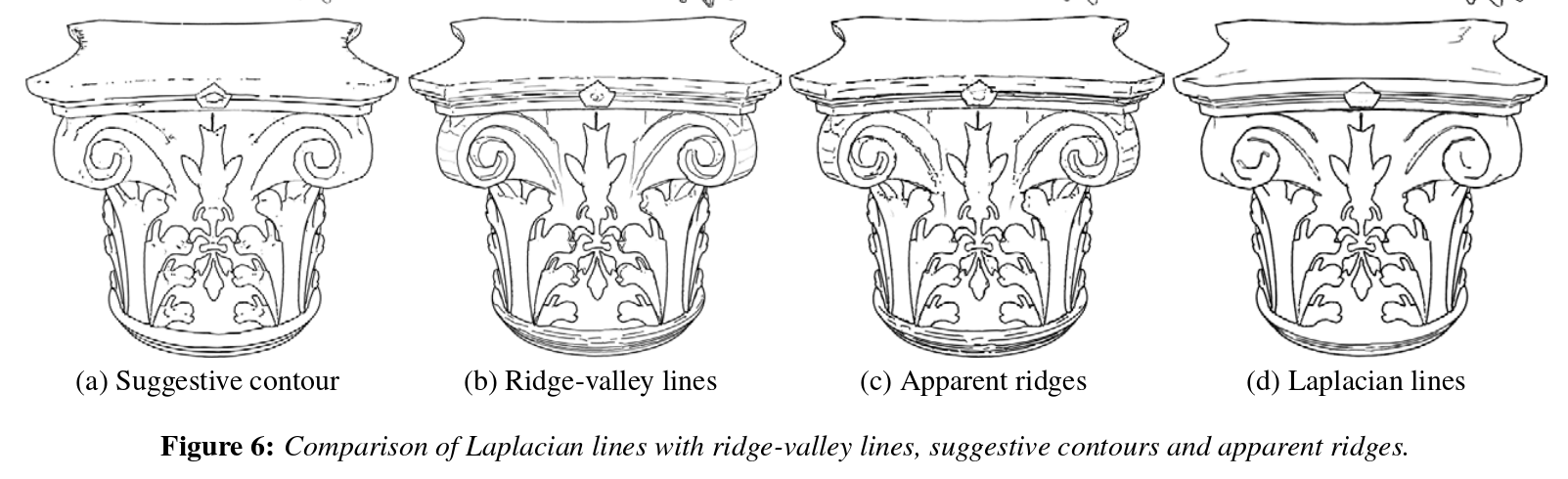
Higher order shape lines. They find more Sharp edges, surface ridges and valleys, and surface inflections, are all surface lines, but differ in order.
Lines we won’t cover
The subject is vast enough as is, so there are some line types we won’t really cover how to detect in this part, but you may still apply the same stylization techniques on them by treating them as arbitrary lines. These include:
- VFX: In general, you can use lines for VFX if you are creative. You could add hitsparks for instance, or even do rain with them. For this, you should provide a good interface for artists to manipulate them.
- Movement lines (speed lines): these are dependent on how much a given part moves, and are very useful in conveying motion in static mediums, or exaggerating it in animated ones. I would recommend treating them as VFXs.
- Explanation lines: These go a bit further than just games, and are not really extracted but specified. They may get additional stylization like adding arrow caps. I mainly wanted to mention them so that you don’t forget that you can do more than just pretty pictures.
- Hatching: Hatching is a bit of a special case, as it is lines put together to represent shading, and behave more like a texture. I think they should be treated as textures then, which also opens up plenty of other questions that would be outside the scope of this article.
Detection Algorithms
Since lines are dependent on geometry, we can find where they should appear. Different types of lines may be found using different algorithms, and the algorithm choice will also affect how you may style and control that line. Tricky!
Most algorithms may be found in one of two categories, the screen-space ones, and the geometry-based ones. But before that, let’s take a look at some rendering tricks that have been used over the years.
The HACKS
The title is a bit provocateur, but you know we love ourselves some quick and easy wins. These methods have been some of the most used, and are usually born of limitations in the graphics pipelines, sometimes from even before we had shaders. We got a lot more flexibility today, so it’s a bit unfortunate that this is still the state of the art for many games.
Instead of trying to find the edges proper, these methods rely on particularities of the graphics pipeline to “cheat” and approximate the solution quickly or in a simpler way. As such, they can work in the specific context they were made from, but may quickly fall apart in other contexts.
While it is possible to expand upon them, I think you would be better served in those cases by implementing a more proper method directly. These methods shine when you want a quick and easy result, but may lead to very complex setups when trying to compensate for their weaknesses.
Inverted Hull
The poster child of this category, and absolute classic of the genre is the Inverted Hull. By creating a copy of the model, extruding it a bit, and rendering the backfaces, we can make a sort of shell around our model. This does reproduce the Occlusion Contours pretty neatly, which is why it has been used in a lot of titles like Jet Set Radio.

The inverted hull method. Really simple to make (less than a minute!), but vulnerable to artifacts.
This method however presents a lot of limits. The processing cost is somewhat high, considering we are effectively rendering the model twice. It is also very sensible to artifacts, as geometry may clip through the line.
One thing this method is good at however, is that you can get some nice control over the colour and width of the line. The latter can be achieved in several ways, the most efficient of which is by adjusting the width by vertex using a geometry shader. This is the method games like Guilty Gear ([Motomura, 2015] ) use, and is a very good way to control this intuitively and avoid some of the artifacts. However, this adds another necessity: the normals of the model must be continuous, otherwise you may get holes inside your hull.

How inverted hull works, using a side view to illustrate. You’ll notice that the hull itself has inverted normals, therefore you only see its “backfaces”, giving the contour line.
Overall, this is a nice method and a smart trick. It has some good basic control on the line’s visual aspect, and is simple to put in place, which can make it pretty useful even with its flaws. However, there is one final flaw which I haven’t directly brought up: this method ONLY finds Occlusion Contours. This means that, to find the other line types, you must use other methods.
 Inverted Hull for Sharp Edges
In fairness, you can, but...
That’s not entirely true, as you can still use a similar method to get the sharp edges for instance, which is what Honkai Impact did. This however requires an actual preprocess step not far from the geometrically-based lines we will see later, which means it will only find the edges that are sharp at preprocess time, and won’t update with the object’s deformations. This means that the method works best for rigid transformations (only affected by one bone), like objects, and not so well for organic parts.
However, if you are making a preprocess part in your pipeline to get those edges, you are losing a lot of why you may use the inverted hull in the first place, which is the technical and time barrier. By implementing this, you pretty much prove that you have both, and could have used that to implement another method that may have suited your case better.
For Mihoyo’s use case, considering they DO use another method for their environments, I believe they did this for a few reasons:
- The characters are excluded from the environment linework thanks to their already working inverted hull, which means they would need to add an exception in their algorithm for objects on the characters.
- For coherence’s sake, since those lines would have the same aspect as the regular inverted hull lines.
- They might have been able to implement this directly in the DCC with something like geometry nodes, and then be able to manipulate them the same way as the existing contour lines.
- The investment to implement a simple line detection algorithm versus one that would cover all their use cases is quite big, especially as they already have their pipeline working as is.
If you are in a similar situation, you’ll probably be better served by a screen-space extraction method, which we will see below!

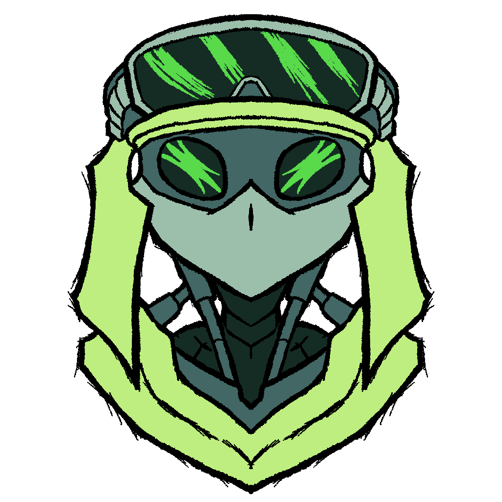
Two examples showing common artifacts of the inverted hull. On the left, a basic IH use, note the lines on the left headphone and collar extending beyond the object, the lines on the glasses stopping before the end, the chin having unstable width, clipping on right headphone and necklace. You can minimize them if you put in the work, as apparent on the right image where the artifacts of the forehead and the collar are much harder to notice at a glance. (Source:Left: Bomb Rush Cyberfunk, Right: Granblue Fantasy Versus Rising)
As a side note, you can also hack together some janky contour lines quickly using the Fresnel factor.
 Fresnel Lines
Want to learn a bad method?
Another method for contour lines is Fresnel / Rim Lines. This uses the fact that the Fresnel factor is related to how “side-on” you’re seeing a surface, which is correlated to the fact that most contour lines are gonna be around “side-on” surfaces, to draw some part of the model in black.
The main flaw here is that word: “most”. This is very affected by the geometry, meaning that you may either get a huge line, or no line at all, depending on the object. I don’t recommend using it, but I find it interesting to mention.
An example of Fresnel lines. The width is somewhat controllable, and you may smooth out the object, but they are really affected by the geometry.
Complementary Lines
The other types of lines being independent of the point of view, they tend to be prebaked onto the model. Yes, this is effectively Arbitrary Lines methods, used to approximate some other types.
Intuition would tell you to just draw on the model, and be done with it. This works, but the line may present a lot of artifacts and appear aliased. This is why you can find two methods to do that.
One of them has become popular because of its use in Guilty Gear, owing to the fact that it’s one of the first commercial projects to have nailed the anime artstyle and being one of the few known complete workflows. I am talking about the Motomura Line, which has been brought by Junya C. Motomura.
The concept is simple: you still draw the line as with the previous method, but you align your texels with the geometry (id est, you make it horizontal or vertical). This alignment will prevent aliased texels from changing your line.
The main issue of the method, is that it is very manual, and adds a lot of pressure on the topology to make it happen. This is not ideal, as topology is already under a lot of constraints, especially for stylized rendering, and having one find a middle ground between shape, deform, shading, and lines, is going to make it harder.
You may see some people use Square Mapping to refer to that. I don’t really like to use that name for the method, because it sounds more generic, and that concept may be used for things outside of lines. I also don’t think it should get a separate name, because it is just an extension of UV mapping, but hey that might be just me.
Another method is to just do it geometrically, just put some quad or cylinder to make that line. It works, but it either makes the line’s width vary with the viewing angle (quad) or extrudes the line a lot (cylinder). This also opens up clipping issues.
But, by using one of those two methods, you may thus have a more complete render! This is how a lot of higher end stylized rendering productions are made currently.
Funny methods from the graphics programmers
All the methods we described earlier have been artist-developed, and came a lot later in the history of rendering. But, even before that, some cool early programmers also looked for ways of rendering lines, with even more restrictions, but also a direct access and understanding of the pipeline.
Nowadays, these methods are not as useful since we know how to do better, but I think it is interesting to show them, especially as you won’t really see them mentioned outside of really specific contexts.
One of them is called the Hidden Contour by [Rossignac and van Emmerik, 1992] , and is kinda analogous to the inverted hull. Here is the trick however: here we don’t add an additional mesh, we will change the rendering parameters to draw the same one again! Here are the changes:
- We render only the backfaces. This is slightly different from the inverted hull, which inverted the normals, thus allowing backface culling to become frontface culling.
- We offset the depth to render in front of the mesh. This means the backfaces will clip a bit in front of the mesh, which then will create that line.
I find pretty interesting to see how the same concept as inverted hull gets implemented when going at it from a programming side, but this also means we got the same need to render the other edges. However, this is programmers we’re talking about, before we even really had DCCs, which means they tend to look at more automated solutions.
This is where what I’ll call the Hidden Fin by [Raskar et al, 2001] comes in, which can detect sharp edges. You create, under each edge, two small quads. They share their common edge with the edge they are testing. Their dihedral angle is set at the threshold the user sets, and is independent of the geometry itself.
What this means, is that if the geometry is flatter than the hidden edge, it will stay hidden beneath the surface. However, if the geometry is sharper, the edge’s quad will show though the mesh, displaying the line!
This is a geometric way to represent that test, which is find super cool! It’s not really the most practical in terms of rendering, because it does require a LOT of geometry, but it’s a nice concept.
Nowadays, the additional control we have allows us to have more robust drawings, and better optimizations, but this is pretty smart and interesting to see!
Why use them?
So why did I mention all of these methods, if better ones exist? There are several reasons, one of them being that I think it’s cool, but it was also to address their use.
These tend to be the most known methods, and are mentioned in a lot of places, but with not a lot of context. Now that you have a better framework to see the limits, you should be able to know when to use them effectively.
The main risk with hacks, is when you try to extend them beyond their field of application. They can be pretty fickle, and you may very well be over-engineering solutions to problems that already have some. This will consume a lot of time, and may lead you to worse results than if you used another of the methods I will present here.
Another reason why I showed them, is that the method may be used elsewhere with good results. For instance, the inverted hull can be used to make some nice looking two-color beams! Another use is to make some parts, like eyes, easier to make, but then that becomes a hack for shading (which I might address in a future article, but hey one at a time).

However, an unfortunate fact at the time of writing, is that getting access to the other methods may be sadly beyond the reach of most people. Indeed, the other ones require nodal or shader programming, and can really depend on the final graphics engine. A lot of the currently available engines don’t really open up their graphics internal, because it’s a very complex subject, but here we kind of need it.
While the algorithm may be easy-ish, integrating it into an engine can be very tricky. I really can’t fault people for not shouldering the cost of implementing these methods and just using a hack. I can certainly hope it becomes less and less as time goes on, so that we can get cooler renders!
Screen-Space Extraction (SSE)
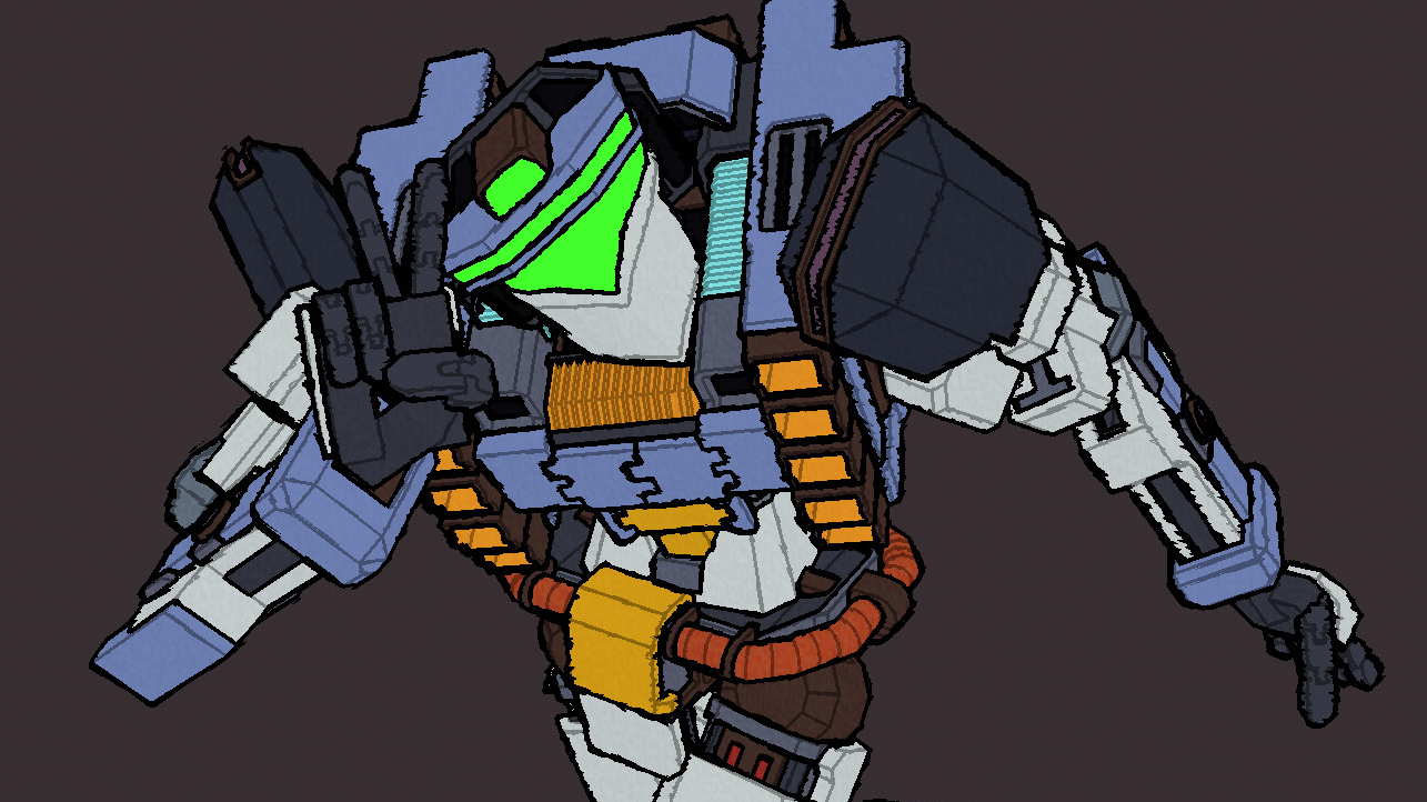
My own game, Kronian Titans uses more advanced SSE methods to give the lines more texture. I’m still not done iterating, but I like how it looks!
Next up is the current standard method: screen-space extraction (SSE). This family of methods boasts the quickest basic speed of all, while being able to detect a lot more line types, but are trickier to control and have some trouble with the control of the width. They are also a bit more complex, which can make them quite limited or tricky to implement without opening up the graphics engine.
The method is based on an algorithm known as convolution: for each pixel, you do a weighted sum of the surrounding pixels, and output the result. Which surrounding pixels and their weight is known as the kernel. This might be a bit tricky to understand if you don’t already know it, so you can expand the boxes below. Convolutions are pretty good at edge detection if using the right kernels, and even a simple Laplacian can get us pretty far.
 Convolution Example: Occlusion Contours
Direct example
A convolution is basically a mathematic way of comparing neighboring pixels. You have a small pattern called the kernel, centered on the pixel you want to compute, where each pixel has a defined weight. You then use those weights and pixel values for a weighted sum, and then use the result as you wish!
Let’s use an example with a Laplacian Kernel, which is a simple way to find the differences between neighboring pixels:
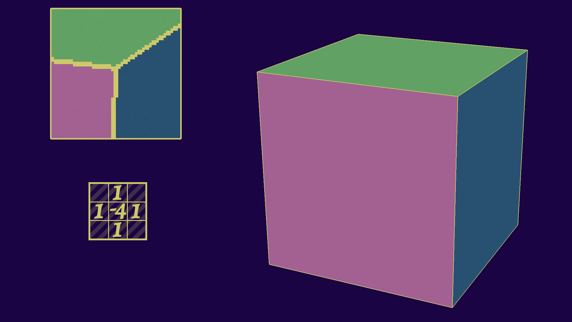
A 3x3 Laplacian kernel is pretty simple: you make a cross of values 1, except for the middle which is -4.
This is equivalent to taking the center pixel, multiplying it by -4, and then adding the 4 directly neighboring pixels (up, left, down, right). What the formula does, is basically compare the center pixel to the average of its neighbors: if it is close to zero, it means they are nearly identical.
We can use that together with a threshold to find discontinuities, areas where the value changes quickly, which is exactly what we need to detect edges as we will see in a bit! If you want a second example about convolutions in general, you can check the other box.
Convolution Example: BlurringGeneral example
Blurring is a somewhat simple operation to understand: you want to average the neighboring pixels. A naive algorithm will probably have a loop accessing all relevant pixels, like this:
|
|
This is functionally identical to what a convolution would do, with a 3x3 kernel, where every value is 1/9, as you can see on this schema:
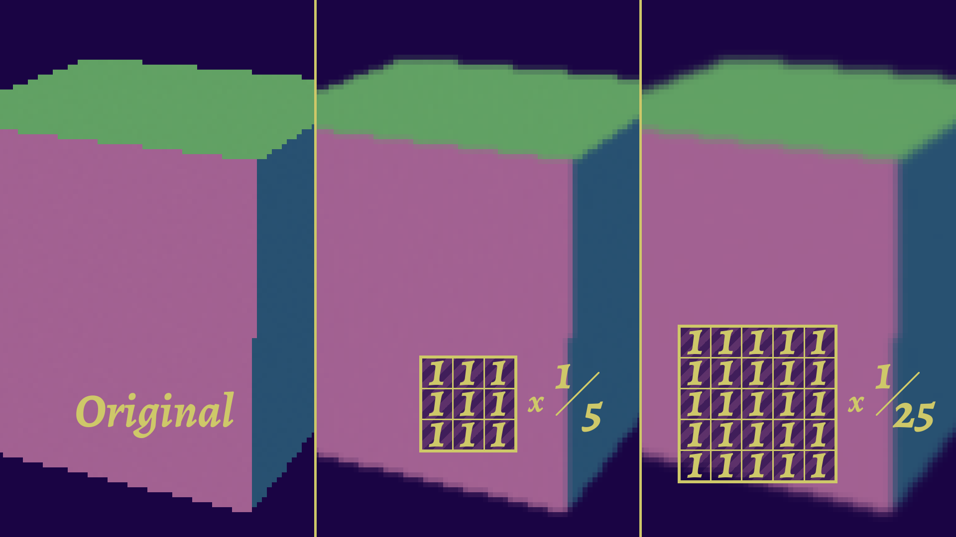
The advantage here is that you can adapt the weights in an easier way. And now it’s math so you can do more math on them!
There are a lot of applications (like neural networks) and subtleties to convolutions, as they are also good at edge detection. Doesn’t that sound useful for our use case ?
The key to understanding this method however, is to realize that we don’t do our convolution on the regular output, but on the internal buffers, sometimes even custom made for this pass! This is what allows us to get good precision and better results than, say, a filter. We can thus make several convolutions on various buffers and combine them to get advanced results:
 What are filters?
A filter in this context is an image processing algorithm that runs on the rendered image, not internal buffers. The advantage is that they may be applied to images from any source. The disadvantage is that they have more trouble finding the parameters from the final image itself.
They tend to be a lot more involved and expensive, but also tend to provide a lot less control, working more like a black box that will output the stylized image. This is the main reason why I think they are ill-suited for games. They also tend to not really keep a coherent stylization from one frame to the next, although that depends on the algorithm.
Similarly, you may have seen a lot of machine learning methods floating around, and while there are many ways to apply it to rendering, you might be thinking of those automatic stylization ones or style-transfer using GANs. While cool, they tend to present the same problems of regular filters, but turned up to 11, so I wouldn’t recommend that direction either.
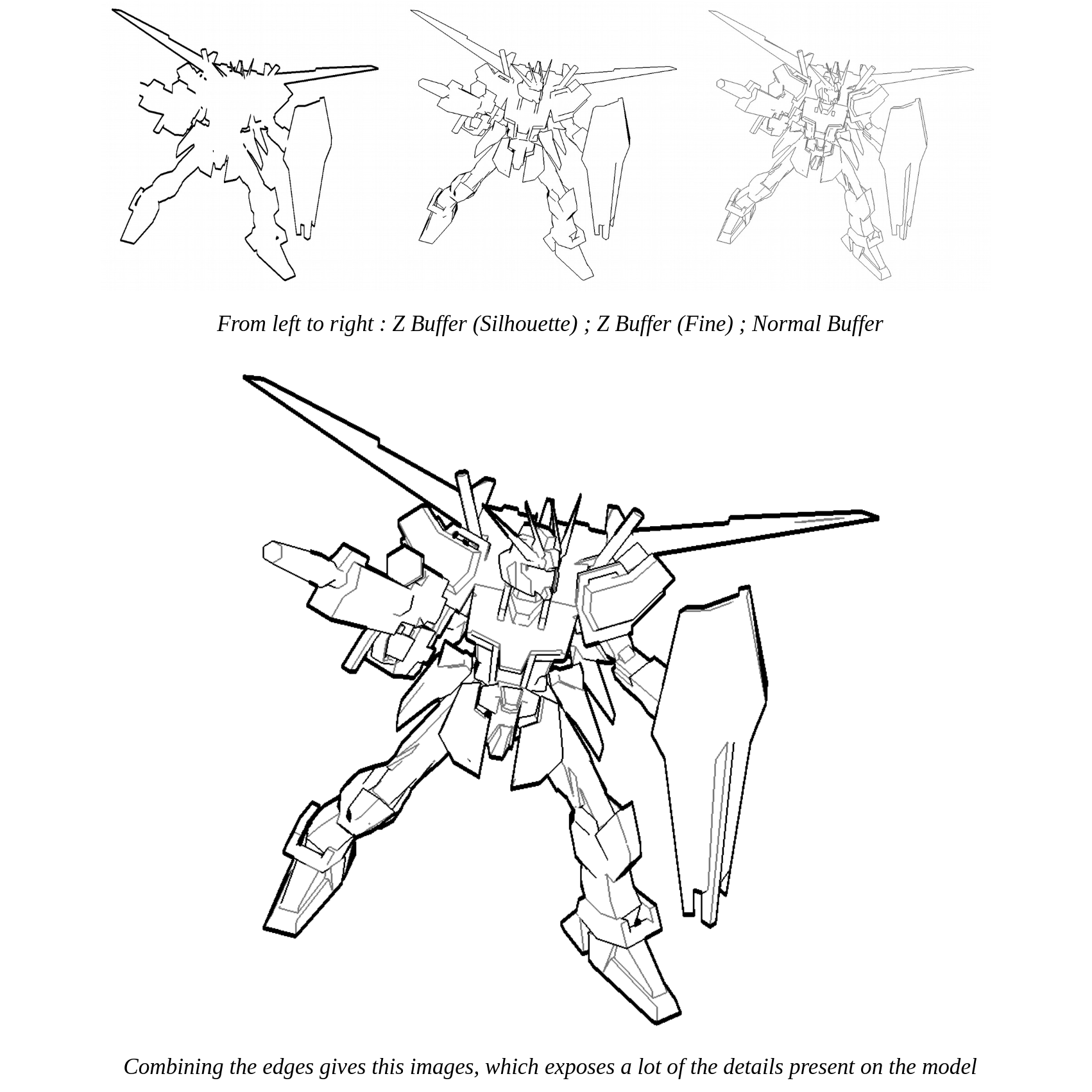
Here, by combining three convolutions together (silhouette, occlusion, and sharp edges) and styling them a bit differently, we can get a pretty nice linework for a very light computation cost. Fun fact: this is in fact among the first shaders I ever programmed, all the way back in 2016!
The fact that it’s screenspace also helps the lines feel coherent at any scale, which you would need to compensate for with the previous hacky methods. Overall, this is a really good method that can also scale with your added demand for control and style, although each step makes the solution more complex. If you get out of this article remembering only one method, this is the one you’ll want to use in most cases.
Let’s now take a deeper dive into the subtleties and various aspects of the method.
How to detect lines depending on their type?
I touched a bit quickly upon that, but convolution is only one part of the answer, the other being the internal buffers we use. The answer will depend once again on the type of line we want to find, so let’s take a look through them once again.
- Occlusion Contours: Considering they are depth discontinuities, we can estimate this from the depth buffer. We look at the central pixel and the neighboring ones, and if the difference is big enough we deduce that there must be two different objects (or at least parts) in front of one another, and select that pixel as part of the contour.
- Sharp Edges: These are surface discontinuities, which means we want to do that with the normal buffer, as this will show us the surface directions.
- Material Separation: Once again pretty similar, but this time the buffer we will need to use will be the material ID buffer, which is a bit less standard and more implementation dependent.
It’s a lot simpler than it reads if you watch it visually. Combine results for a complete linework! In order: depth, normals, material.
So that’s our easy lines out of the way. Let’s continue with some trickier ones.
- Silhouette Lines: This can be done in a few ways. A simple but flawed one would be to use the depth buffer again, with a higher threshold. This kind of works, but won’t strictly find the silhouette in all situations, with both false negatives and false positives. Another way could be the alpha channel, but this requires that your object is rendered separately (so more useful for pipelines). The better method would be similar to material separation lines, as it would be an object ID buffer. This would allow us to cleanly separate objects, but might not always be accessible by default.
- Arbitrary Lines: Once again, there are a few ways to do so. One way would be to rely on the same technique of using some sort of ID buffer once again, more specifically a custom ID buffer. This would be a simple method, and may be combined later with width control to create independent lines, which is what Tales of Wedding Rings VR did. Another could be rendering those lines directly in the buffer, but that may require a more advanced pipeline control. This is the kind of method I use for Kronian Titans and Molten Winds.
- Shadow Lines: This can be done through a specialized buffer, which we may call the shadowing mask. It is usually an intermediate result of a computation, but by exporting it like this you may detect those straightforwardly.
- Other Lines: The method may be extended further again, by using some other buffers that may be computed, but can be less pertinent depending on what you want to do. One classic example is for instance outputting the depth of only the characters to a separate buffer, then compare that buffer to the regular depth buffer. If the character is further away (and thus hidden), you may trace a silhouette around it to see it through walls!
The method can detect most types of lines, especially mesh intersection (through object ID buffers) and shadow lines, which are very tricky geometrically. It might however have some difficulties with higher order lines (which would be expensive to compute).
This may be pushed further through the use of custom buffers and shaders, depending on the type of data you are manipulating. This can either be used to optimize your detection, by packing all the needed values inside of one buffer, or by outputting specialized values (like the shadowing mask). This is in fact what Kronian Titans does, by combining its three ID-based detections into a single buffer.
In this part of the article, as I am still only talking about extraction, I am styling all the contours the same for simplicity. Know however that as you find each contour separately, you can also flag them separately, and thus style them separately. You just have to include that functionality when implementing your shaders.
Improving the precision
Now, that’s the base idea, but we might still get a few artifacts. This section is about how to improve our results a bit. This is not always applicable to all line types.
Glancing Angles
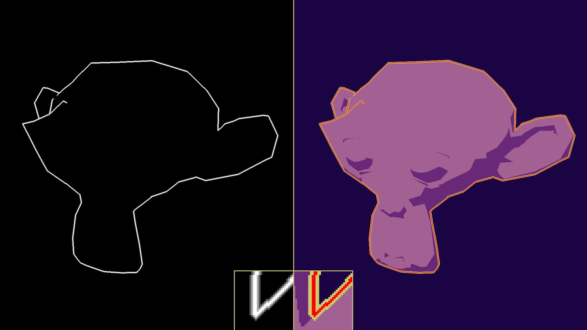
The first order of business is going to be improving the threshold, which is very useful for contour lines. Indeed, since we’re using a flat threshold, we are just looking for an absolute difference in distance from the camera. This usually works, but can break down at glancing angles, and you may find false positives. However, increasing the threshold wouldn’t work either, because it might miss objects that are close together.
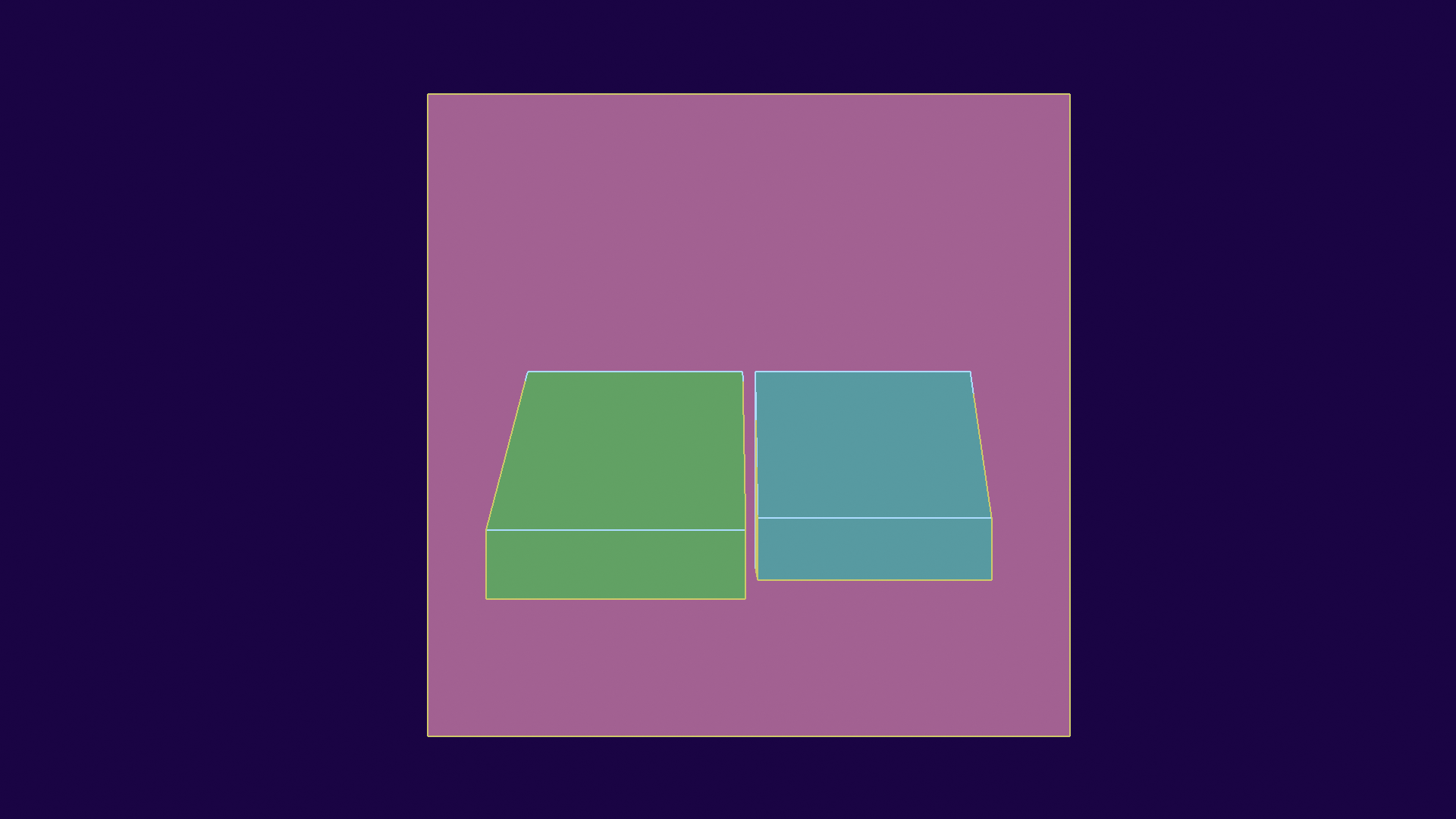
Here, it’s easier to see in an image:
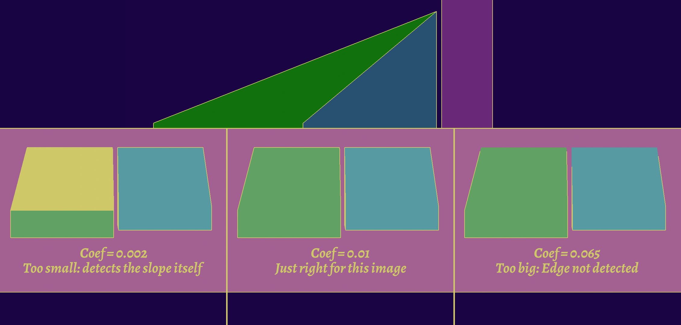
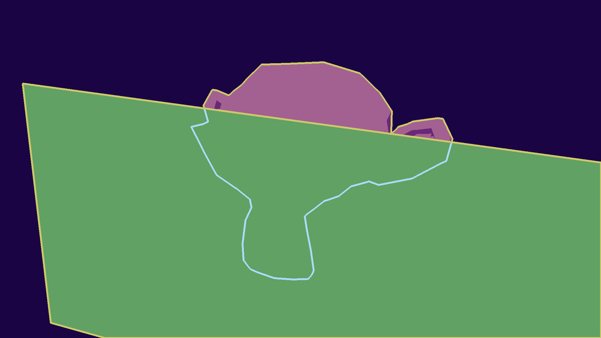
Here it is shown with an angled plane, but it can happen on almost any model. This is hard to fix directly because it is very dependant on the viewpoint.
One solution would be to adjust the threshold depending on the slope of the surface, which we can know by taking the normal at the central pixel. The exact formula depends on implementation.
Unfortunately, this adjustment might make us miss lines we would otherwise find. It’s a fundamental limitation of screen-space extraction algorithms, as we may only rely on information we have on screen. The main way to improve this would be to use several detection methods at the same time, but this might bring some limitations in the stylization part.
Several Detection MethodsCombine and win!
As it can be common, sometimes the best solution isn’t an algorithm that can handle everything, but a combination of specialized algorithms.
In this case here, adding more detection will reduce the conditions for this to happen. So for instance, detecting normal discontinuities will find the previous example, but not faces that are parallel. Another way would be to use object IDs, meaning as long as it’s two different objects, it will be detected.
This is not to say that they don’t have failure cases, but by combining them the remaining failure case is really hard to come by: you need that the two faces are parallel AND very close AND part of the same object for the line to not be detected, meaning the artifacts are going to be very few.
Here we have an inappropriate depth threshold (too high, doesn’t detect all lines), but it is compensated by the sharp edge detector. As you can see, this can still result in artifacts depending on the exact style you use.
Other Kernels
Another way to improve detection is to use different kernels. Right now, we’ve been using a simple Laplacian kernel.
The classic has been to use Sobel kernels for edge detection. It’s actually two kernels, one vertical and one horizontal, that you combine the results of. Compared to Laplacians, this catches some edges better on the diagonals, but also slightly more expensive, as it requires 9 texture accesses compared to the 5 of a simple Laplacian Kernel. The dual kernel nature also means you can use only one of the two directions to only get vertical or horizontal edges for instance.
An addition to that has been Scharr kernels, which are optimized Sobel kernels that handle diagonals better and are tailored to the hardware limits. For instance, where a regular Sobel kernel will use the coefficients 1, 2, and 1, the Scharr kernel for 8 bit integers (incidentally, a color channel in most images) are 47, 162, and 47.
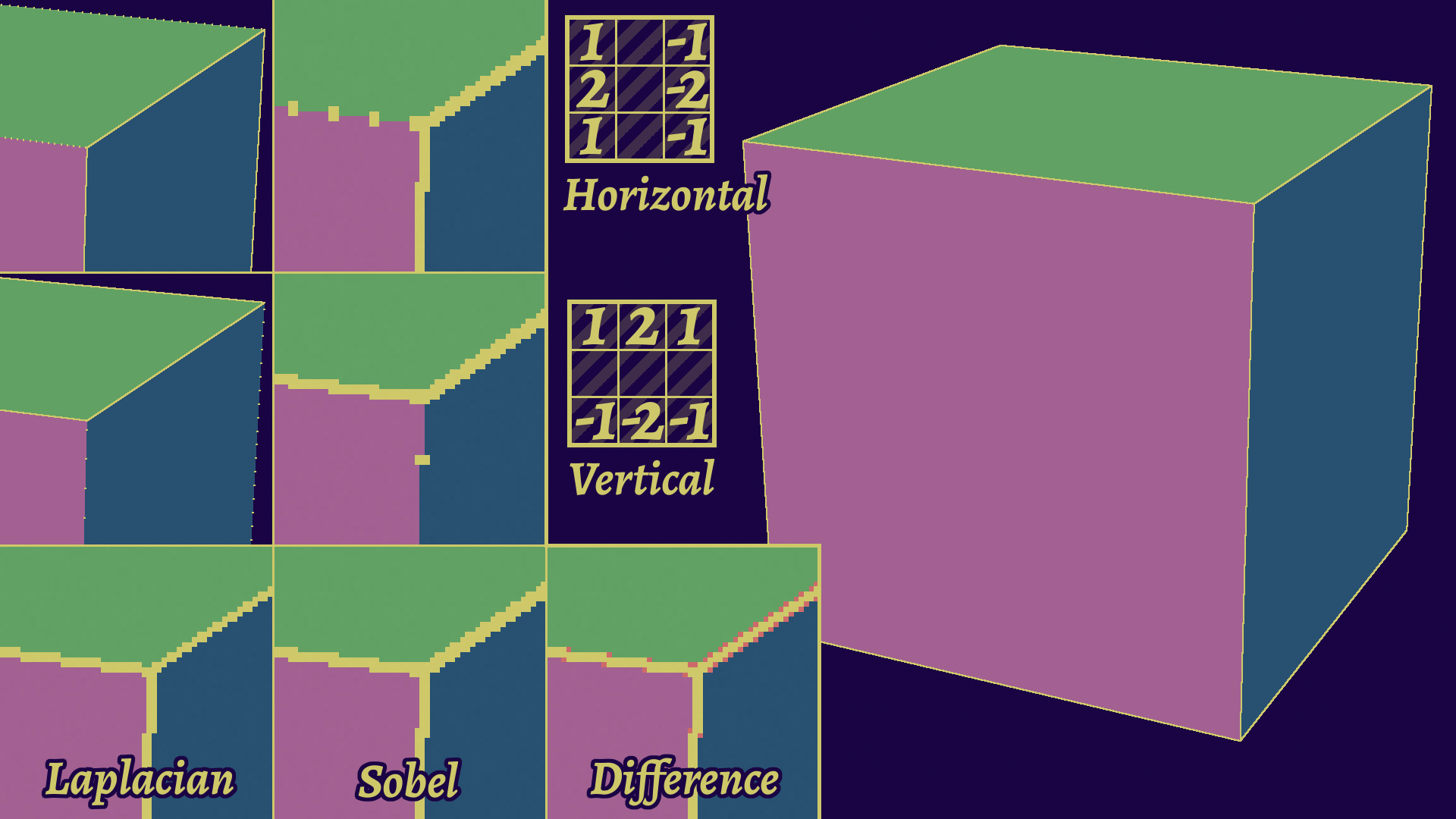
3x3 Sobel-kernel based line detection and comparison with a Laplacian kernel. Sobel is the combination of a vertical and horizontal convolution, and is a bit more robust to diagonals. Scharr would achieve the same result in this simple example.
There are, of course, other edge detection methods, which are outside the scope of this article. Some examples include the Canny edge detector, or the Difference of Gaussians operator. They tend to deliver better results for photographs, but can be a bit (or very) slow, and trickier to pass parameters with, so I prefer sticking to the simpler ones.
Something to also note here is that I’ve only presented 3x3 kernels, which is in my opinion sufficient. But, if you want to go for bigger kernels, like I don’t suggest you do in the next part, you can find more suitable coefficients online.
The question of width
At this point, we have a way to detect lines, but the issue is that our lines are all the same size of one or two pixels (depending on if you’re using absolute value or not). This is problematic because it limits the amount of styles we can express and our ability to remove specific ones. This is actually two problems, one of them is actual control which we will see in the next section, and the other is enabling it, which can be tricky in screen-space extraction.
We can now detect lines, however an issue remains in that our lines are all the same size of one or two pixels! This is problematic, because it limits the amount of styles we can express and our ability to control it. In order to unlock that, we will have to start by being able to have thicker lines.
One might get the idea to start using bigger kernels to detect lines from further away. This actually works, and you have two ways to do it, but each have flaws.
- If you are using a full bigger kernel, your rendering is going to slow to a crawl as the number of samples increases sharply (it’s O(n²) after all) with each pixel of width you want to add, making even medium-thin outlines hard to fit in a real-time game.
- If you are dilating your kernel, it will reach further, but you’ll get a bias and loss of precision as you go further. You may also miss lines locally and thus have them displaced. This can be fixed by adding more samples, but you start getting closer to the first method.
There are a few additional tricks to these methods including rotating the kernels, but bigger kernels naturally tend to have some noise in line detection, as you may detect features that aren’t local to your part, which might translate into artifacts.
Dilatation
In order to avoid these problems, we can use dilatation algorithms, which expand a line using a kernel. The basic idea is just that, they’ll check the whole kernel and if they find any pixel of the line, they’ll expand.

“The dilation of a dark-blue square by a disk, resulting in the light-blue square with rounded corners.” - Wikipedia
This is naturally a lot more precise, as you keep the detection local and then make those lines bigger, but a naive implementation will be just as long as a bigger kernel. Therefore, we will prefer using several dilatations one after the other, which can be often implemented using ping-pong buffers.
While you could start thinking about what is the most optimal number of passes and kernel size for a given width, I’ll cut to the chase, since we can solve that problem with the Jump Flood Algorithm. The basic idea here is to sample from further away at first, and then halve the distance each time. This allows us to dilate more with each step, making the algorithm log2(n), which in layman’s terms means “very very fast”. If you want to know more about the implementation of such an algorithm, this article by Ben Golus will interest you.
At this point however, you might have noticed that we still widen all lines homogeneously. This isn’t enough for the control we want to achieve, therefore we will need to compute what’s called the SDF (Signed Distance Field). To simplify, this is about computing the distance to our line instead of a flat “our line is here”, which then means we can adjust it or do cool effects.
The SDF (on the left) allows us to control the line width and style, as is shown on the right (simple two color line).
Thankfully, computing the SDF is very easy with line dilatation methods, so we don’t have to change anything really for those. The methods using the kernel technically can, but it’s kinda hacky.
 Kronian Titans' SDF Line Detection
How to go beyond engine limits
To illustrate, this is what I’m using in Kronian Titans. It IS slower and less precise, but it allows computing the SDF in a single pass, which is pretty useful in Godot 3’s limited renderer.
The idea here is somewhat simple: you sample in a pattern, but associate each sample with a distance. Then, you take the minimum distance of all the samples that detect a line.
This method is very affected by the pattern choice, as more samples is more expensive, while less samples will introduce bias and provide less precision. Ideally, you want a rotationally robust kernel, or even rotate it to limit that bias. I would also force the closest neighbors of the pixel to be checked each time, to ensure you don’t miss lines. Kronian Titans uses a variation of the 8 rooks pattern I did manually.
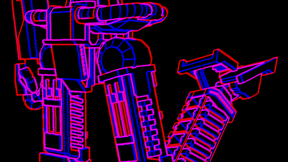
The line detection buffer of Kronian Titans. You can see the bias there, but hey it works in real time and doesn’t need to open up the renderer to do, which is good enough for now.
There is a small point remaining, which is about if the base line is one or two pixels wide, but this will be explained better in the next chapter. I’ve also mentioned it in my GBC Rendering article!
Best overall choice for Games
Kinda spoiling the article hehe, but yeah I believe that at the moment, Screen-Space Extraction algorithms are the best choice for games. For offline rendering, it’s a bit debatable with the next method.
In my opinion, it’s a bit hard to argue against, really:
- They can find pretty much any line type that you want.
- They are the fastest.
- They can do a fair amount of stylization options.
- Their main flaws, like limited width, can be corrected with some elbow grease. (Okay, not always easy, but doable in most cases)
Hacks’ only advantage here is that they are easier to implement, which may be unfortunately a breaking factor for your team, and that’s okay. It’s a bit unreasonable to ask to open up the renderer and code a ping-pong dilatation algorithm inside a complex game engine, so I hope this becomes easier as time goes on. We will see how to implement all that in part 3.
SSE algorithms have however one fatal flaw: stylization can be pretty hard or limited! This is especially true for a simple common case, which is pretty hard with SSE: lines that change width as they go on! This is where the next family can help us.
Geometry-Based (Mesh Contours)
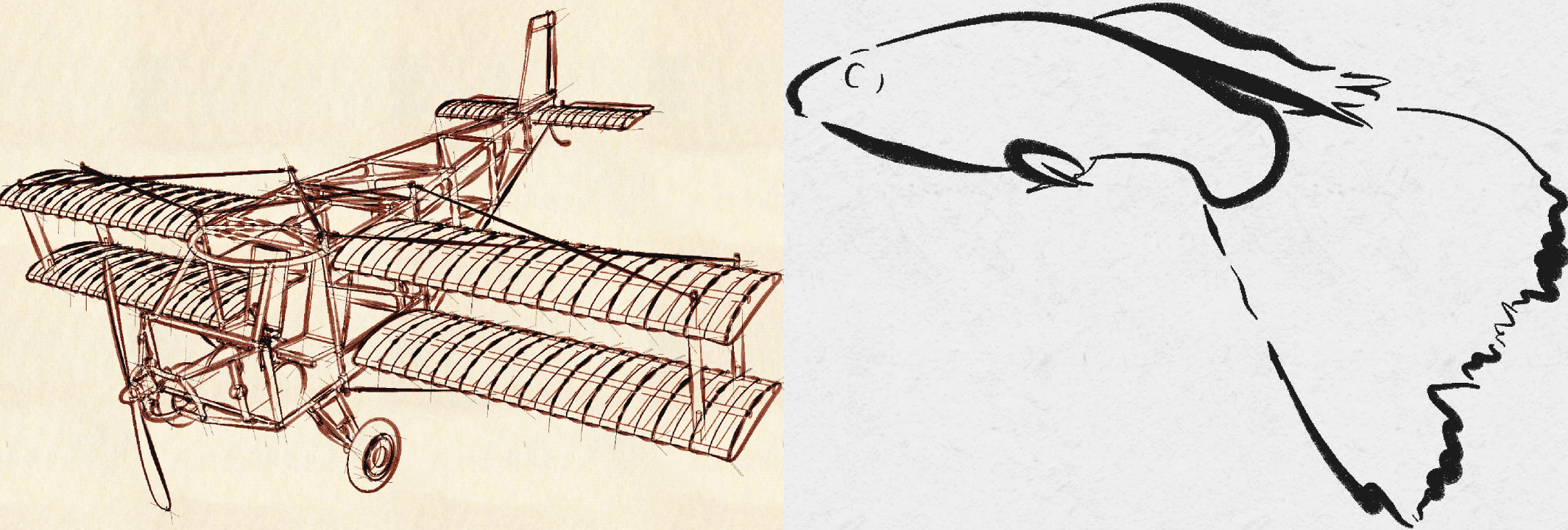
3D renders from [Grabli et al, 2010] , using different styles. This method allows us a lot more freedom in rendering!
Hey! 2025 Panthavma here. This part has been completely rewritten, because this was my PhD subject! My work has changed the landscape in regards to its realtime application, so it’s worth a re-read if you’re coming back!

And finally, the last method: mesh contours! These work by analyzing the surface itself, edge by edge, and extracting lines that way. I have no video game example, but you might have seen them in Blender Freestyle.
The biggest difference with other algorithms is that you have line primitives, as opposed to independent pixels. This unlocks a wealth of additional options, like varying the width, combining or simplifying lines, drawing them with textures like dashed lines… There’s a lot!
It’s also got higher quality, with extermely precise detection that leads to a lot less caveats. Combined with a better direct control potential, it’s really the most promising method! If you have it, you can really expand your horizons, both in terms of possibilities and in terms of production speed, as you can achieve higher quality with less effort.
So… why isn’t it used? There’s several reasons, but the main one is very direct: it’s REALLY slow. You have to iterate over every edge of your model! Do you know how many edges a regular AAA model has? If you do, you’re a big nerd since it’s not a stat that matters in 99% of gamedev contexts, so I actually got a few and checked: it’s around 300k edges. Even if your algorithm is processing one edge in one nanosecond, that’s still 0.3ms for a model, and you got several of those. And you got other steps after that one to actually render the lines.
I could go on about technical direction for a while and the tradeoffs you can make, but I’ll give a quick reference point. A 60FPS game needs to render a frame in 16.6ms, but you want some buffer so that the spikes don’t tank it, so make it 13ms. On many games, your regular opaque render is 7-8+ms, add maybe 1-2 for transparency. Your full budget for post-process is closer to 3-5ms in practice, and you would be blowing it all on line rendering that can’t even cover the whole scene!
The other reasons are more classical. The first one is the classic stylized rendering issue: there’s not a lot of info that most people that would be interested can access. I guess this article is part of the solution then! The other one is that it’s quite hard and time consuming to implement, so the cost is really prohibitive, even moreso due to the mandatory optimizations.
In this part, I’ll address the technical landscape of the first part: extracting the lines. The full algorithm has 3 additional steps, but these are better suited to the next parts of this series, since they relate to the stylization of said lines. (No ETA there, there’s many open questions I need to organize my thoughts on first)
Detecting Lines
Extraction is mostly straightforward, and almost always involves compairing the two faces adjacent to the edge to find the geometric property you want. You’ll need a winged-edge data structure (the 4 vertices and the two face IDs) to do that efficiently. The nature of the algorithm being a very simple procedure but heavy on volume makes it perfect for GPU.
I actually did a very in-depth implementation guide for this, but it’s still in a weird published-unpublished limbo, so I’ll explain it in my true voice when I can in a full article!
Following this is a list of edges you can detect with this method. There’s an additional point: the method will detect hidden lines. This is both a boon and a curse, as you’ll need an additional visibility pass, but that’s for the next article. This makes mesh contours uniquely suited to some applications and styles, usually closer to technical drawings.
- Sharp edges may be found simply using the dihedral angle of the two faces. If it’s sharper than a threshold, detect the line.
- Material separation is also similar, by comparing the material ID of two faces.
- Arbitrary lines are already extracted, so you just need a way to mark them.
- Boundary edges, which are edges with only one neighboring face, are trivial.
- Illumination lines is very simple for simple flat shading, by using the face normals to compute lighting. It is somewhat simple for smooth shading by using the vertex normals, but you’ll need to use a variant called interpolated contours. However, normal maps are very tricky to use in this context, and way outside the scope of this article.
Extracting inside of faces: Interpolated ContoursA variant that's good for math but bad for games
An alternative algorithm to testing edges is testing faces, by using the geometric normals at each vertex and then using linear interpolation to find the accurate edge. This is an extension of using triangular meshes as an approximation of a smooth surface, which they are meant to be.
Note that I wrote “geometric normal”, not “shading normal”. This specific algorithm doesn’t take normal maps into account.
This does produce cleaner contours, as there won’t be any bifurcations, but this also bring a lot of potential issues, like contours being found behind the triangular mesh. This does require a lot of additional adjustments and potentially artifacts for no real gain. Therefore, for the rest of this article I’ll only focus on triangular meshes.
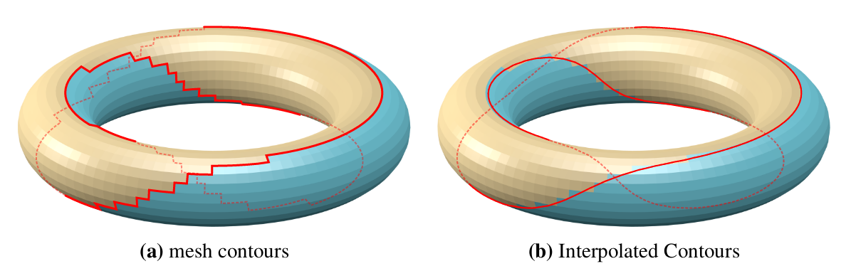
Mesh contours vs Interpolated contours. You can see the line go through the backfaces, which means it will be hidden if no precautions are taken. (Source: [Bénard & Hertzmann, 2019] )
- Finally, Contour lines. Let’s dive into it.
Contour extraction is going to be the complex part, as depth discontinuities are not local. We can thankfully use other geometric properties, by defining a contour edge as a point where the normal and view direction are perpendicular. We can express it in simpler terms however: if one face faces the camera, and the other faces away from it, it’s a contour edge.
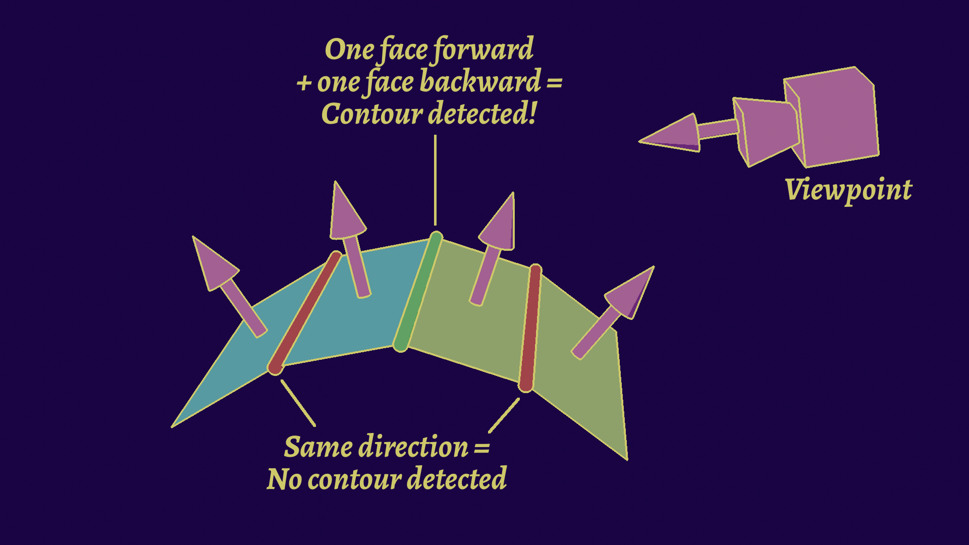
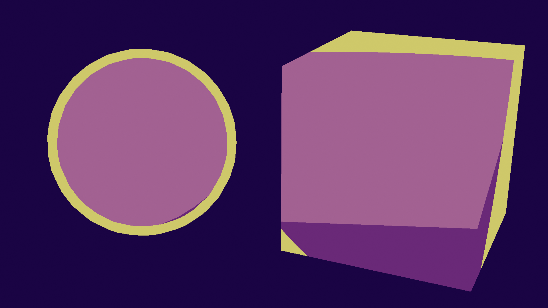
Compare the signs of the dot products of the view direction and the faces’ normals.
An additional step you need to make is to recompute the view vector from any point on the edge and the camera’s position. This is only needed for perspective projection, as the deformation will alter the exact contour edge for the picture. While this seems small, it actually complexifies a lot of the optimizations later on.
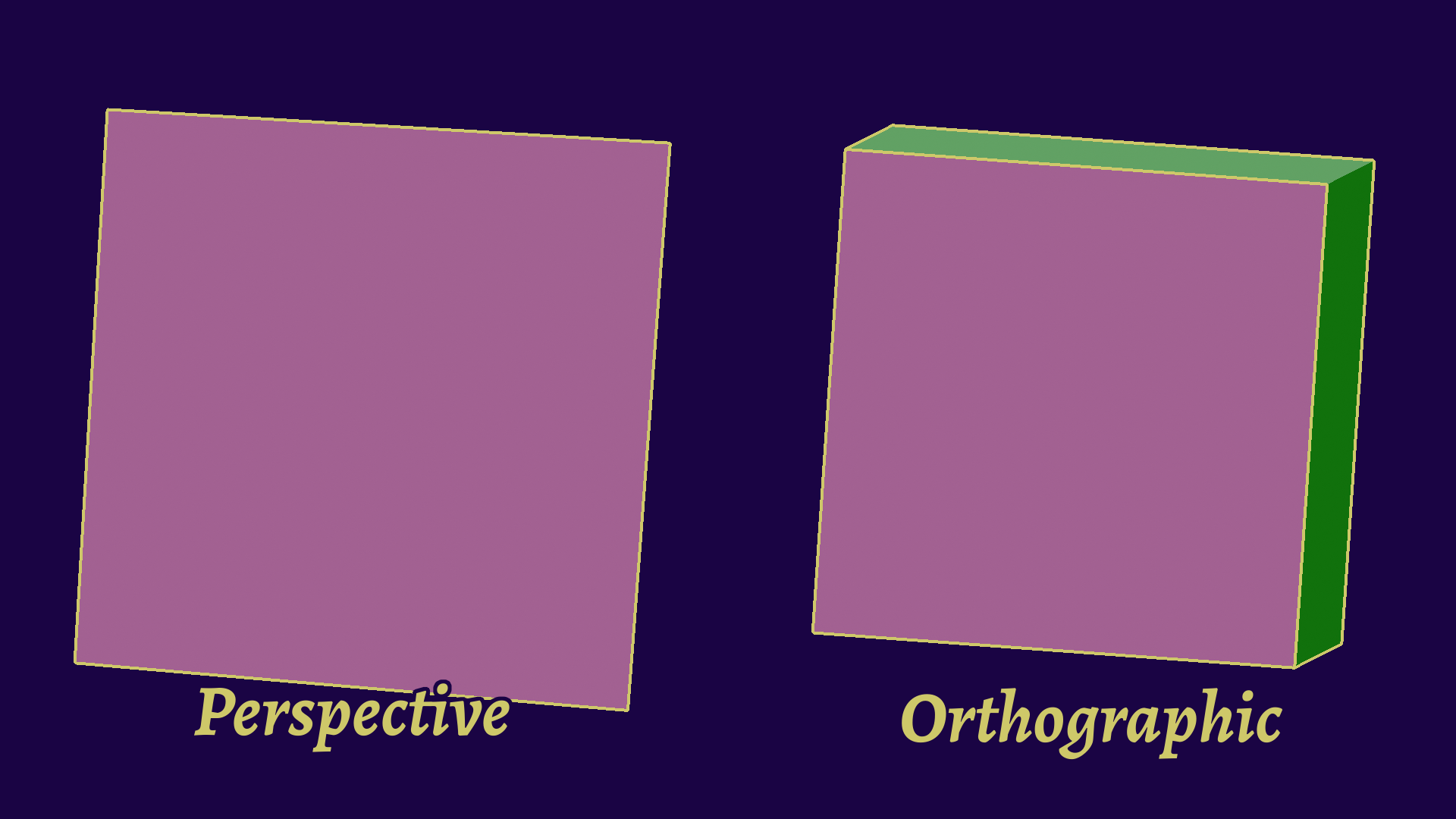
The same cube viewed in perspective (left) and orthographic (right) projections. You can notice that the actual contour changes, which is why we must recompute the view vector.
Do note that there is one type of line that mesh contours can’t find easily: intersection lines. These are one of the strengths of SSE methods.
Model Intersection LinesIntra- and Inter- model detection
Again, not exactly true but you’ll suffer if you try to implement it. Geometric algorithms don’t care about intersections at this step, only focusing on their own little part at a time. Finding these lines will require you to take the whole model into account to find self-intersections, and the whole scene for general intersections. This is also another family of algorithms, collision detection.
Compare this to SSE algorithms, where it’s just comparing two pixels on an object ID buffer to find inter-model collisions. Self-intersection is a bit trickier, but by default you’ll still find discontinuities, and between material IDs and sharp edges you’ll very probably have a line at that intersection.
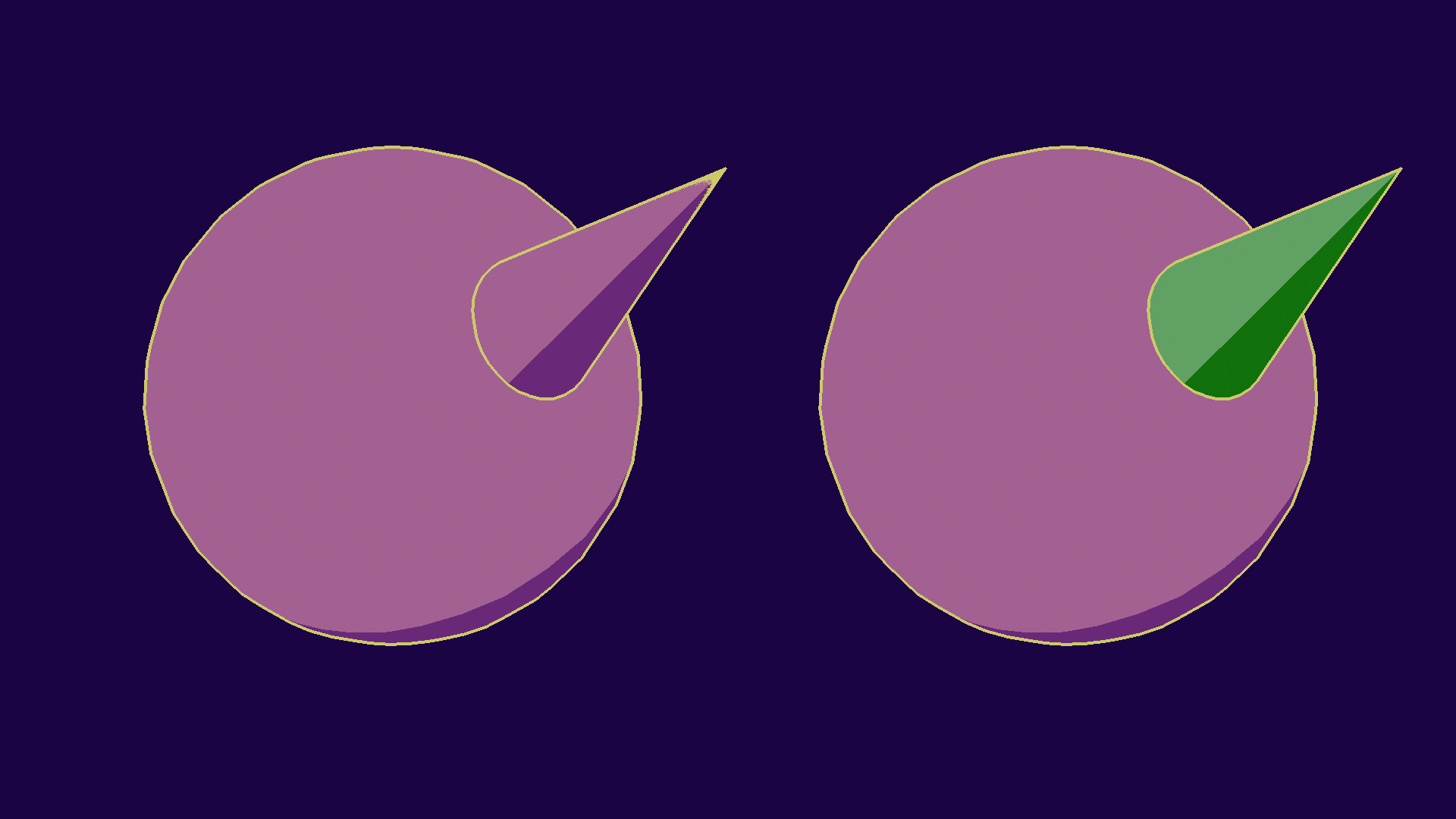
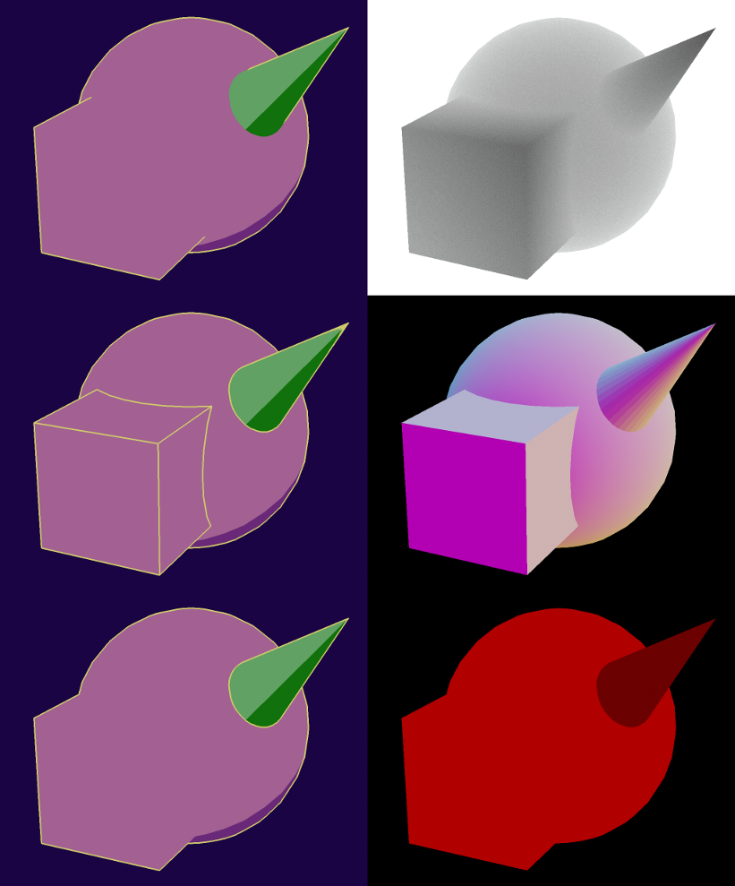
Self-intersection on the left, and inter-model intersection on the right, both found using SSE methods. You’ll notice that using different IDs limits artifacts along the spike.
And with that, we’ve seen the base algorithm. You can program a basic bruteforce implementation now! But, now comes the tricky part: making it realtime.
Optimizations
Now’s the tricky technical part… but I won’t go into it in depth. Each of these is available in full research papers, so I’ll give you the gist so you get a basic idea of what exists.
There have been a good few optimizations for mesh contours, but they tend to have one or more of these issues:
- Randomness: Some implementations are not guaranteed to find all edges, and just edge their chances to find most of them. I don’t like that personally.
- Static: Optimizations that don’t often target only static meshes, which means environments. When I did my research, there was nothing for characters.
- CPU focus: Not a lot of GPU-adapted implementations exist, so data structures can be inefficient.
To understand the following optimization, a few properties of contours will come in handy:
- The smaller the dihedral angle between the two faces (i.e. the sharper it is), the more probable it is to be a contour.
- Inversely, no visible contours may exist on concave surface, so we can filter them out beforehand.
- Contours are sparse, often around the number of faces to the power of 0.5~0.8, which means we can get very big speedups if we can guess correctly where they’ll appear.
- Contours tend to be next to other contour edges.
Temporal Methods
When we want to make more than one image, we may take advantage of the fact that contours don’t move that much when changing the point of view slightly. This means that so as long as the camera isn’t making wild movements, we can use the previous frame’s contours as a starting point, and explore from there.
This will raise the likelihood that we find contours quickly, and thus we may even be able to stop the algorithm early if we are running out of time with potentially good enough results. Additional edges can be prioritized depending on their distance to a found one, since contours tend to be together, and small movements may cause slight position changes.
Similarly, we may also start our search randomly on the mesh, and prioritize edges close to where we have positive matches. This allows us to more quickly converge on the result and stop the search early, although you may still miss some edges.
Overall, these methods are a speed up strategy that you may leverage over time to ensure fluidity, at the cost of graphical artifacts.
Static Methods
A few methods rely on constructing acceleration structures to make finding the edges faster, by limiting how many to check. I’ll present two of them here: Cone Trees, and Dual Space. The issue with those methods is that their construction is slow and specific to a given geometry, meaning that the mesh can’t change after this, limiting it to environments.
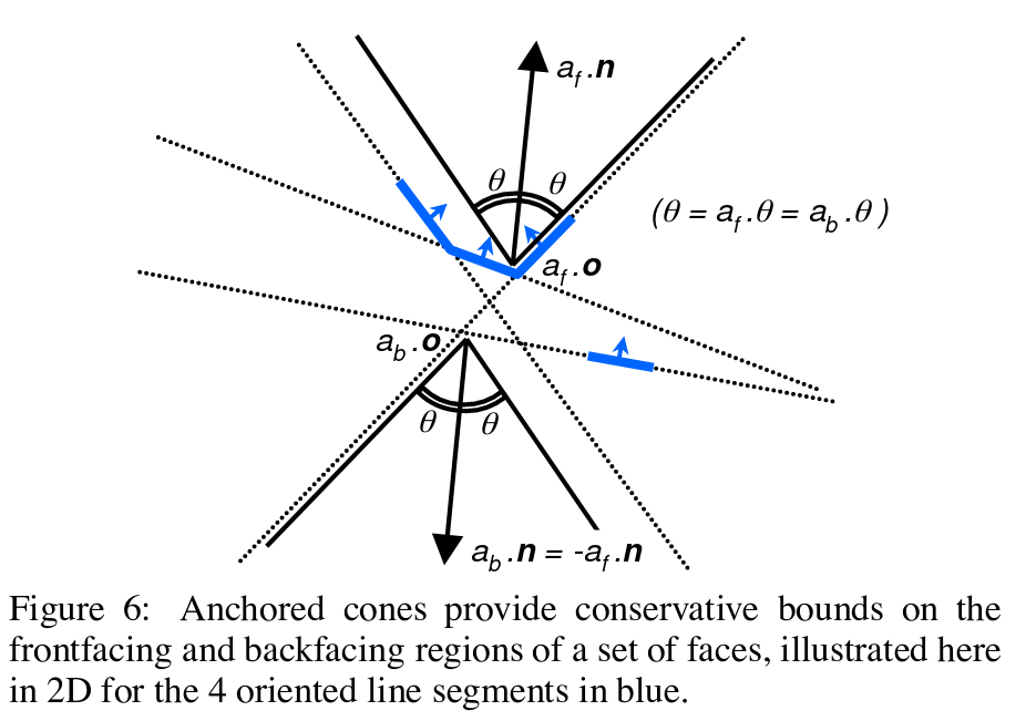
First up is Cone Trees, which has been described in [Sander et al, 2000] . The idea is grouping faces together into patches, in order to filter a lot of edges at once. This is done by making a cone for each patch, and checking the normal against it instead.
These cones are stored in a tree data structure, which must be constructed beforehand, as it is quite slow, but you may be able to discard more than 80% of your edges in this step!
A patch along with its cone. Notice that the faces are not necessarily adjacent. (Source: [Sander et al, 2022] )
Next up is Dual Space and Hough Space methods. This one’s a bit scarier, so I won’t go into too much mathematical detail, just the basic concepts.
Let’s start with the dual space transform. For graphs, like meshes, the dual graph is a graph constructed by making one vertex per face, and edges for adjacent faces. For our needs, we will also set their position to their normal, leving us with this:
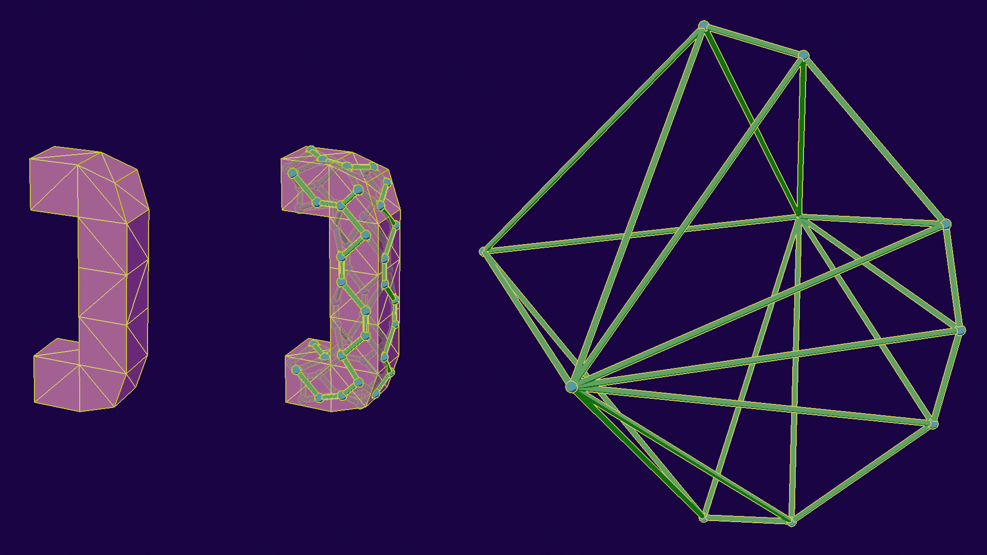
Illustration of the process. Left: original model, Center: Dual Space, Right: Projected Dual Space
Now that we have done that, we can find contour edges by creating a plane perpendicular to the view, and looking for intersections between it and the edges. This effectively changes the class of the problem from “comparing all normals” to “look for geometric intersections”, which we know to optimize better with specific data structures, like BVHs!
This is however where the perspective transform rears its head again, as the view vector will be different every time. Thus, in order to make that, you need to add an additional dimension, making it effectively 4D collisions conceptually.
In order to improve this, [Olson and Zhang, 2006] have suggested using Hough space for the computations, which has a benefit of being more uniformly spread along the BVH, speeding up traversal.
All these transformations take a lot of time, and as such must be done as a preprocess, which increases complexity. Those structures are not really adapted to the GPU either, as their hierarchical nature will often encourage divergence.
My Method
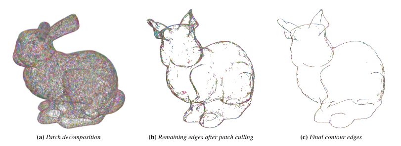
Teaser figure from my research paper ([Tsiapkolis and Bénard, 2024] ), showing (a): the initial mesh, (b): what remains to be tested after my culling step, and (c): the actual contours. As you can see, it’s already quite close!
To solve this issue, I ended up developping a new method that takes all of these constraints into account. The results are really good! You can see more details in my research paper ([Tsiapkolis and Bénard, 2024] ) itself, although I’ve got extra performance tips in my PhD manuscript.
The way I did it was to create a flat structure derived from the one [Johnson and Cohen, 2001] introduced, the Spatialized Normal Cone. This is very similar to the other static methods (it is in fact one of them) where you group edges into patches, but my contributions come mostly in HOW I make those patches and how I adapted to character models. Most of those improvements are made possible by advances on the mathematical theory behind it I made, including a more precise and flexible definition of the structure, and an alternative test to find the contour.
Adapting to charactersTLDR I'm sidestepping the problem, but it works
Alright, cat’s out of the bag… My method doesn’t really solve the character problem. What I do is simple: I detect the rigid parts, meaning the ones where only a single bone is used. That means for instance, the back, the middle of the leg, the skull, are parts that often don’t change much, but joints like the elbow or knee tend to not be rigid.
On a rigid part, you know that the angle of the faces won’t change, so you can confidently make patches, and remove concave edges. Non-rigid parts skip that culling step and are bruteforced instead. The performance impact depends on the overall rigidity of the mesh, since the optimization factor will only happen on those part. According to my test set, this seems to hover at around 50% rigidity for classic organic humanoid meshes. Different modelling methods may change that ratio, especially in stylized rendering.
A consequence, to the surprise of no one, is that my method works really well on mechas and robots which tend to be very rigid (98+%). Since these are the coolest type, the method gets extra points.
To understand what makes a patch good, meaning that it leads to better performance, we must first see which criteria we have to optimize:
- The flatness of a patch, as the flatter the surface the less likely it is for it to have a countour edge, meaning you can discard it more often.
- The smallness, as due to perspective transform this will affect the potential view directions and thus we’ll need to check more patches. This is the bounding volume on SNC, but I’ve managed to prove that you could use a smaller volume.
- The number of edges, as you want to discard more edges per patch… but each edge make the other two parameters worse!
It’s impossible to bruteforce this problem even on simple meshes, and it’s hard to evaluate a patch, so most methods ended up separating edges based on one parameter first, and then the second one. This introduced bias into the build process, leading to potentially worse performance. My big contribution was figuring out a formula to that ties all of these together, which combined with a measure of the time required to compute a patch and an edge, allowed me to compare patch computation times directly.
I then used this formula to assemble edges greedily. I start by creating one patch for each edge, then compute what fusion will give me the best performance boost. I then continue until there are no fusions that will increase performance, so I do find a potential local maxima!
This can then be used on the GPU in a simple two-pass method: first pass does the culling, second computes the edges. The flat data structure makes this doable and fast, although you do need to take care with your implementation as the time scale is very small.
I skipped over a lot of details here since this article is an overview of the domain itself. The questions you might have like ‘does the measure step make it computer dependant?’ (it’s negligible in practice) or ‘how long is the preprocess?’ (basic implementation is slow, but accelerations are possible and quite fast) are probably already answered in my paper and/or my PhD manuscript, as well as a very likely future article on this blog focused on the method!
Is it ready to use? Not really…
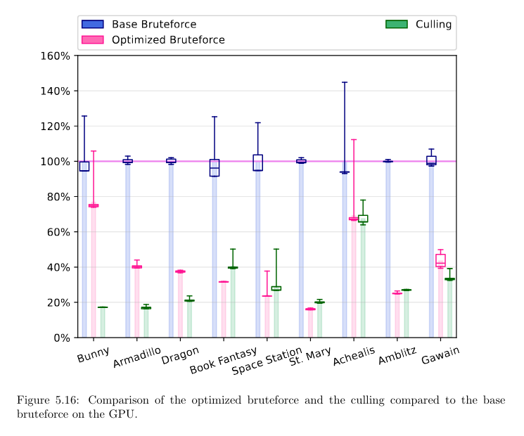
Excerpt from my PhD manuscript, where I compare the normalized performance of a good but basic bruteforce implementation (which means, something that’s properly parallel and with regular buffers) to my optimized bruteforce (whose limit was the lab computer’s power supply) and to my full patch culling algorithm. Having all that together can allow you to START thinking about implementing this in realtime, and you’ll still have a lot of work.
So… Is it usable in realtime now? YES! I’ve proven it. Is it ready for use? Erm, not really.
There are many points that still need work. First of all, that’s only the first step of the pipeline. What are the next ones?
- Visibility is the step where we find which lines are actually visible, and which ones aren’t. This is the flipside of being able to detect invisible lines, and it’s not trivial, as lines may get cut midway through by another object, so we need screen-space intersections.
- Chaining comes after, and is the process of taking our individual edges and putting them together as part of a larger line. This helps us unlock more stylization options.
- Finally, Stylization (and rendering) is the last step of our pipeline. This is where the fun is, but it is also more complex than it seems!
This is beyond the point of this article, as I’m only covering that first step this time, and will cover these in this series in a later article. If you want to learn more, I suggest you read [Bénard and Hertzmann, 2019] which is a very complete state of the art, and [Jiang et al, 2022] which has a realtime implementation of those steps on the GPU!
On top of that, we have no standard in control, so there’s also a lot of work to be done on artist tools, as otherwise you can’t really access all those improvements. That’s not just an article for this blog, that is a whole series to dedicate to that open question!
Finally, a huge obstacle, even if you’re willing to explore that space, is simply that the implementation cost is HUGE. You would have to implement that whole set of optimizations, which is not easy. Something I didn’t go over is how much actual low level optimization I did. My bruteforce was so fast, the limiting factor on the lab computer was actually the power supply, and it still just kinda makes the cut for heavier applications! The base bruteforce in the above figure is already a good implementation, naive ones can be 10x slower than that!
And after that, there’s the difficulty of putting it into a game engine, which varies wildly between which one you chose, but it’s the kind of algorithm that’s pretty far away from what you usually do in these engines, so it’s an additional high cost. All of this, together, makes it that it’s often not worth the cost for most teams. It’s something you need to buy into early, and spend months on tech, and I can’t recommend it over the other methods at this point unfortunately.
So… Is the dream dead? Well, I said most teams, but at this point I feel I’m familiar with the subject, have the skills, have the opportunity, and my project Kronian Titans would really benefit from it, so… get on the newsletter to not miss what I’m cooking?
In Summary
I hope you enjoyed reading this article! It took quite a while to make, and that’s after I split it into three parts! We saw quite a lot, so let’s quickly review what we learned:
- People tend to draw lines based on the objects’ geometry, which means we can teach the computer to detect them.
- A few hacks exist to get results quickly, but are limited. They should be used knowingly, and you should know to level up from them when the need arises.
- Screen Space Extraction methods are the current standard. They are fast and pretty complete, but you’ll need more advanced development to really unlock their potential.
- Geometric Extraction methods can unlock high quality lineart, but they are tremendously hard to use right now. This is what I’m working on!
There’s a lack of resources online that really explain these kinds of topics in-depth, so this is an attempt to make the situation clearer. People are often blocked from making cool looking games because of a lack of technical and general knowledge of stylized rendering subjects, so if you’re in that situation I hope this article finds you well!
When to use each algorithm?
Here’s my general recommendations, which you may use as a starting point:
- I don’t have artists in my team: You’ll want a SSE algorithm, as you don’t have the bandwidth to adjust lineart properly. Simple one works, more advanced one can make your scene look better “out of the box”.
- I only have non-technical artists in my team: Inverted hull is probably going to be your go-to, but a mild inverstment may get you a SSE shader with some control, which might save you time in the long run.
- My project needs high quality lineart: I think a more advanced SSE algorithm would be the way to go, with plenty of controls available. We’ll see how to in the next articles of this series.
- My project needs high quality lineart and I only have non-technical people: This is starting to get tricky, and you’ll need to choose between taking a lot of time for each asset with inverted hull, or invest in your pipeline with and advanced SSE algorithm (by skilling up or getting a technical person)
- I only need lines for one small thing: This will depend on what, but inverted hull for objects, and SSE if it’s an effect (like outlining the player through walls)
Of course, this is very simplified. The more complete recommendations are going to be in part 3, but this should already give you an idea.
Next time!
We only looked at the first step today! In the next articles of this series, we will see other aspects: Stylization of those lines, Control Interfaces, and Practical Use! There’s a lot that can go wrong in these implementations, and a lot of knowledge that’s very dispersed and not easy to link together, so I hope you’ll be there with me for the journey!
In the meantime, you could do well to register to the newsletter to not miss it when it releases! I also talk often about these subjects, so you can also join my Discord or follow me on Twitter!
Alright, see you in the next one!
Bonus Reading
Here are some additional parts if you want more! They either didn’t fit in the article properly or were too specific.
Raytracing and ReflectionsNot super adapted funnily enough
So I’ve talked mostly about video game rendering, but not so much about offline (comics, movies, etc). To be fair, most techniques apply the same, except you don’t care about runtime performance as much and it’s easier to implement.
A big difference for these, is the fact that offline renderers tend to do raytracing, which doesn’t really work with SSE, which is why they use the rays as a first step to reconstruct an image. For the other families, it tends to be similar to the real-time version.
Something that raytracing can do pretty well however is reflections and refractions, and this is supported by those line algorithms, but since it’s pretty niche I won’t expand on it further in this series.
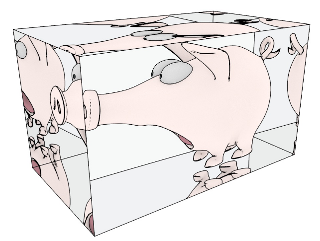
Lines inside of reflections and refractions from Ogaki and Georgiev (2018). Pretty interesting!
Mesh Contours and 2-ManifoldnessReal world data isn't that way
It’s quite a specific detail that will only come up for people that DO implement it, or geometry processing nerds that immediately clocked it when I said “winged edge structure”. Or you want to 100% read the article!
A mesh is called 2-manifold when each edge has at most 2 faces attached to it. It’s not the full definition, but it’s good enough for practical computer graphics like our purpose here. This property does affect a lot of algorithms, and mesh contours is one of them. After all, how do you handle when an edge has 3 faces? Which ones do you compute? How can an edge be both contour and not contour?
Here’s how I handle it in practice: I ignore the issue.
By that I mean that I’ll just generate an edge per face pair. Game models are almost never 2-manifold, and some more advanced stylized modelling tech will take advantage of that. The points on which it happens are rare enough so the performance cost is low. That also makes sure you don’t miss an edge. Boundaries are already handled as a special case as we’ve seen before.
Bibliography!
- [Cole et al, 2008]: Interesting study on where people draw lines!
- [Motomura, 2015]: One of the most known workflows for stylized rendering, which is now used in a lot of productions.
- [Rossignac and van Emmerik, 1992]: Hidden contour method!
- [Raskar, 2001]: Fin edge method!
- [Vergne et al, 2011]: SSE method, introduced line order definition
- [Ben Golus's article on wide outlines]: Good technical article on SDF implementation for lines!
- [Bénard & Hertzmann, 2019]: A very comprehensive state of the art of mesh contour rendering!
- [Grabli et al, 2010]: One of the main papers for mesh contour stylization!
- [Jiang et al, 2022]: Very recent paper on realtime mesh contour stylization. The custom rasterizer is pretty cool!
- [Sander et al, 2000]: The paper that introduced cone trees!
- [Olson and Zhang, 2006]: An article on hough space contour extraction (similar to dual space).
- [Johnson and Cohen, 2001]: Another article on an acceleration structure for contour extraction, which I based my own paper on!
- [Tsiapkolis and Bénard, 2024]: My own paper! Shows how to achieve realtime performance on GPU contour extraction on static models and characters. I've got some extra info that's in my PhD manuscript itself.
Updates to the article
- 2025-10-17: Adjusted the article a bit for presentation purposes, rewrote the whole mesh contours section, and added an aside on 2-manifoldness. Replaced the inverted hull artifacts image.